[1] examined how powerful machine learning can look deceptively convincing when the evaluation setup is flawed. However, in spatial prediction problems, such as real estate applications involving capital gains estimation, rent forecasting, or price prediction, the problem does not end with fixing temporal leakage. Even when time is handled correctly, models can still appear far better than they really are if spatial dependence, repeated-asset structures, and uneven regional coverage are ignored. In these settings, the hardest part is often not fitting a flexible model, but designing an evaluation framework that tells us whether the model truly generalizes beyond the neighborhoods, asset types, and market segments it has already seen.
Spatial data increasingly plays an important role in guiding sustainable initiatives. Geographic information can be used not only to assess real estate values, but also to evaluate territorial vulnerability for urban planning and infrastructure investment, optimize logistics and mobility services, improve accessibility, and estimate insurance risk to help prevent major disaster losses, among other applications. In these contexts, geography is not just another feature, it shapes the operational and economic environment in which outcomes are generated.
Spatial data it is not organized like ordinary independent rows. It comes with geometry, proximity, adjacency, and dependence. Nearby places often behave more similarly than distant ones, an idea commonly summarized by Tobler’s first law of geography: everything is related to everything else, but near things are more related than distant things [2]. So, in these cases the modeling problem changes. Training and test samples are not longer independent, repeated geographic units can make forecasting look easier than true generalization, and uneven coverage can make a model appear reliable only because it is being judged on dense, well-observed areas.
Even though, in practice, AutoML and code agents [3, 4] can now automate most parts of the workflow, the hardest parts remain human: understanding how spatial dependence, panel structure, and coverage shape the credibility of the results.
The Spatial Traps
In summary, the goal of this article is to offer practical guidance on the most common methodological problems that make models appear more generalizable than they really are:
- The Proximity and Persistence Trap: a model may appear to perform well on new data when it is actually benefiting from spatial proximity, temporal persistence, or familiar market conditions already presented in the data. This affect training, cross-validation, and parameter tuning procedures that rely on the assumption of independence.
- The Coverage Illusion: when overall performance is driven by large, dense, and well-observed areas, while sparsely covered regions remain poorly understood and weakly predicted.
- The Boundary Illusion: when model quality depends heavily on how geography is partitioned, grouped, or coded, even though those boundaries are often administrative conveniences rather than economic realities.
- Geographical bias: spatial variables may appear highly predictive while quietly encoding deprivation, unequal access to opportunity, or long-standing patterns of segregation, which can lead models to reinforce exclusionary outcomes even when protected attributes are not explicitly included.
- The Hedonic Oversimplification: when visible property attributes are treated as if they were enough to explain value. In housing valuation, features such as balconies, terraces, amenities, size, or accessibility may capture useful price signals, but they do not fully explain the market. Scarcity, regulation, credit conditions, income, employment, and supply limitations can dominate individual preferences, especially in constrained markets.
- The Silent Maintenance Tax: when the excitement of a promising model hides the long-term burden of monitoring, validating, updating, evolving, and defending it once it faces real market conditions.
As spatial data becomes increasingly valuable in many applications, this article aims to list some of the problems that can arise in this type of setting. This is not intended to be an exhaustive list. For a more comprehensive review of ML pitfalls across different problem settings, see [5]; for a broader discussion of related modeling issues beyond this specific context, see a previous article [1].

Proximity and persistence trap
A good model should not only perform well; it should improve on the structure that is already present in the data. In other words, it should beat the right baseline. In spatial problems, this means that a meaningful baseline should capture at least two basic mechanisms already suggested by Tobler’s argument: persistence, where the future tends to resemble the past, and spatial autocorrelation, where nearby places tend to behave more similarly than distant ones.
For real estate, rent, or capital gain prediction, this means that a model can appear strong simply because expensive areas tend to remain expensive, dense markets remain dense, and nearby assets share similar economic and spatial conditions.
In this case, a weak baseline, such as predicting the global mean, may make a model look impressive even when it is only exploiting basic spatial memory. More meaningful baselines should capture what is available, such as the previous value of the same area, the historical average of a neighborhood, the average value of nearby properties, a seasonal naive forecast, a simple hedonic regression, or a basic spatial interpolation method. These baselines are meant to represent the minimum structure that any serious spatial model should improve upon.
In the same way like the chosen baseline has to take in consideration the structure of the data, the validation should make this as well. If the train and test sets are split randomly, nearby observations or repeated geographic units may appear on both sides of the split. The model is then evaluated on places that are not truly independent from the data used to train it. The result is an error estimate that looks rigorous but is systematically too optimistic. Spatial, temporal, grouped, or blocked validation schemes are often needed to test whether the model can generalize beyond familiar locations, familiar periods, or repeated spatial entities.
Example:
To make this idea more concrete, we experiment with the London House Price Prediction dataset from Kaggle [6]. The goal is not to build the best possible house price model, but to show how the interpretation of performance changes when the validation strategy and the baseline change. The target is the next-month median log price within the same area_id + property_type panel.
Table 1 compares two validation settings. Panel A reports a random split, the most leakage-prone setting in spatial-temporal prediction problems, because similar observations from the same locations can appear on both sides of the split. Panel B reports a temporal-spatial holdout, where the model is trained on earlier observations from observed spatial units and tested on future observations from spatial units that were not seen during training. This second setting is intentionally harder: the model must generalize not only forward in time, but also to unfamiliar geographies.
To keep the comparison focused, we use the persistence (time) benchmark as the main reference point. This benchmark carries forward the previous observed value and represents a simple but strong temporal baseline. We then compare it with a spatiotemporal KNN mean baseline, which uses nearby historical observations to capture local spatial-temporal structure, and with two predictive models: CatBoost, as a strong non-spatial machine learning model, and GPBoost, as a spatially informed model that can account for area-level structure. The goal is not to build an exhaustive model leaderboard, but to show how the interpretation of model performance changes when evaluation moves from familiar observations to unseen geographies.
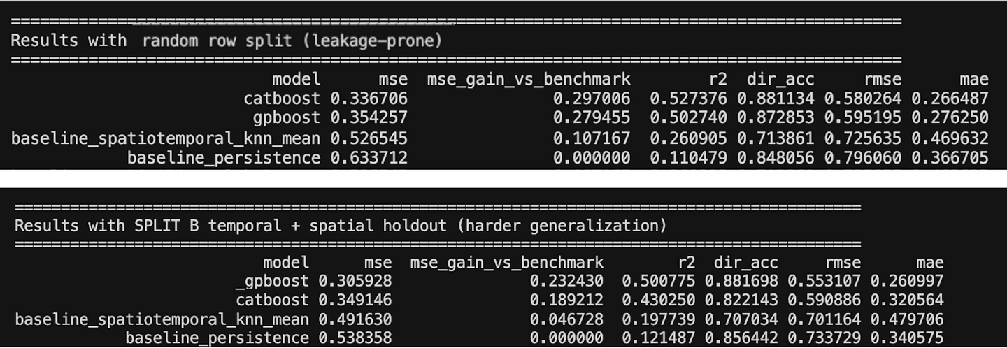
The results in Table 1 should be read relative to the persistence benchmark. The metric mse_gain_vs_benchmark is calculated as the MSE of the persistence baseline minus the MSE of each method. A positive value means that the method improves over simply carrying forward the previous observed value, while the persistence benchmark itself has a gain of zero by definition.
This benchmark is important because the experiment is not asking whether a complex model can beat a weak global average. It asks whether a model can improve on a simple temporal structure that is already present in the data. In real estate panels, yesterday’s expensive areas often remain expensive tomorrow, so persistence is a meaningful first hurdle. However, persistence mainly captures temporal dependence within the same area_id + property_type panel; it does not explicitly model proximity between different locations.
For that reason, the spatiotemporal KNN baseline plays a different role. It uses nearby historical observations to capture local spatial-temporal structure. Together, these two baselines help separate two questions: can the model beat the previous value of the same panel, and can it add value beyond a simple rule based on nearby historical observations?
Under the random split, CatBoost achieves the strongest performance. However, this setting is also the most vulnerable to the proximity and persistence trap: observations from familiar areas, market conditions, or nearby locations can appear on both sides of the split. In this case, strong performance may reflect the model’s ability to exploit repeated local structure rather than its ability to generalize to genuinely new geographies.
The temporal-spatial holdout changes what is being tested. Here, the model is evaluated on future observations from spatial units that were not seen during training. In this setting, the spatio-temporal KNN baseline remains useful because nearby historical areas still carry signal, but the strongest performance comes from GPBoost. This suggests that explicitly modelling spatial structure can be more robust when the task requires transfer to unseen locations.
The main takeaway is the proximity and persistence trap: a model can look strong when random validation allows it to benefit from familiar temporal and spatial structure already present in the training data. The relevant question is therefore not only whether the model beats persistence, but whether it still adds value when familiar geographies are removed from the test setting. Random validation can make the model look good for the wrong reason; temporal-spatial holdout tests the harder and more operationally relevant question.
More to consider:
In spatial settings, cross-validation often fails because observations are linked across both space and time. As a result, conventional folds can create two distortions. During model selection, the hyperparameter tuning process may favor models that exploit residual spatial structure or spatial proxies, instead of models that transfer robustly to unseen geographies. During model assessment, spatial proximity between train and test gives the predictor an unauthorized view of the test environment, making error estimates look better than they really are.
For these reasons, spatial and spatio-temporal problems require validation strategies that separate observations according to geography, time, or both. Methods such as Spatial+ cross-validation [7] and spatio-temporal resampling [8] are designed to make this separation explicit, both when estimating final performance and when tuning model hyperparameters [9].
The Coverage Illusion
In real-world applications, observations are not evenly distributed across time/space. Some areas are densely represented because they have many transactions, many records, or more frequent data collection, while other areas appear only occasionally or are almost absent from the sample.
This matters because aggregate error metrics can hide where the model is actually failing. A model may report a low overall error simply because most of the test set comes from well-covered, high-density regions. In those areas, the model has seen many similar examples before, so prediction is easier. But this does not mean the model generalizes well everywhere. It may still perform poorly in sparse or underrepresented areas, where the local market structure is less visible in the data.
In this sense, good average performance can create a false sense of reliability. The model looks stable because it is being evaluated mostly where the data is abundant. The real weakness only appears when performance is broken down geographically: some regions are well learned, while others remain almost invisible to the model.
For example, bad modeling decisions like removing observations with missing future targets, excluding low-transaction areas, computing spatial aggregates using future information, or selecting only regions with sufficient historical records can systematically reduce the representation of sparse locations. These decisions often improve the apparent quality of the dataset while simultaneously making the prediction task easier. As a result, reported performance may reflect a progressively curated subset of well-covered regions rather than the true geographic diversity of the problem. Coverage should therefore be monitored throughout the entire machine learning pipeline, since every processing step has the potential to alter the spatial distribution of the data and introduce hidden optimism into the final evaluation.
The Boundary Illusion
What looks like a reliable geographical signal may partly be a product of the boundaries chosen for the analysis. Consider real estate prices. A model may use the average price of a district as a geographic feature, assuming that properties inside the same district share a similar market context. But this assumption can be misleading. Two streets within the same administrative district may behave very differently if one is close to transport, schools, parks, commercial activity, or high-demand housing stock, while the other is exposed to poor connectivity, lower liquidity, or weaker buyer demand. However, when the data is aggregated at the city level, these local differences are averaged out. The city may appear more stable and homogeneous than it really is. At the regional level, the smoothing effect becomes even stronger, potentially creating the illusion if uniformity across the whole region.
This is where the Boundary Illusion becomes important. The geographical boundaries used in the analysis (postcode, city, region, etc.) may look natural or objective, but they are often administrative choices.
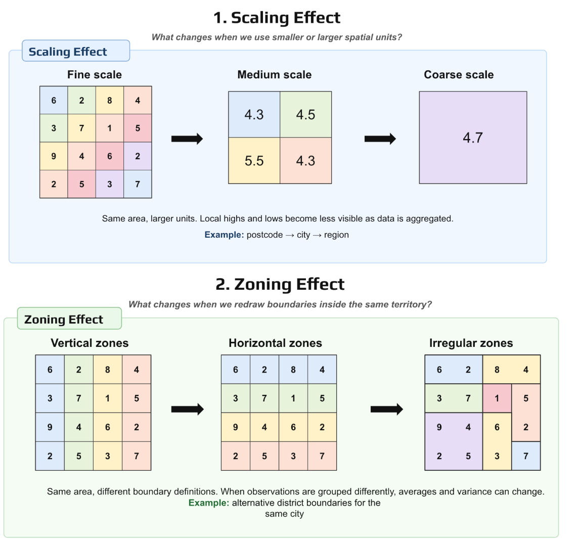
The Figure 2 helps to illustrates this, the top part of the figure shows the scaling effect. The underlying values are the same, but they are aggregated into increasingly larger spatial units: from a fine scale to a medium scale and then to a coarse scale. As the units become larger, local highs and lows are smoothed out. The average may remain similar, but important spatial detail disappears. In a housing or banking example, this means that a risky pocket visible at postcode level may disappear once the data is averaged at city or regional level.
The bottom part of the figure shows the zoning effect. Here, the overall area and rough scale stay similar, but the boundaries are redrawn in different ways: vertical, horizontal, or irregular zones. The observations are the same, yet the averages and variances change because different households, properties, or borrowers are being grouped together. A model built on these aggregated features may therefore change not because reality changed, but because the analyst chose a different way to partition space.
The practical implication is that a robust pipeline should test the same variables and models at multiple spatial scales and, when possible, under alternative zoning systems, to check whether the conclusions remain stable.
Geographical bias
A more subtle problem appears when geography is not only a source of dependence, but also a proxy for social structure. In many real-world datasets, location variables such as ZIP code, neighborhood, census area, branch territory, or regional market are not neutral coordinates. They often encode differences in income and demographic composition.
This creates what we can call the Geographic Proxy Trap: a model may not use a protected attribute (like etnicity) directly, yet still reproduce unequal treatment because spatial features are correlated with that attribute. In this situation, the model can appear technically valid while producing systematically different error rates across groups.
For example, in a insurance fraud referral model, the model may learn that claims coming from certain ZIP codes are more likely to be suspicious because those areas have historically been associated with higher investigation rates, denser reporting, or different claim patterns. Even if ethnicity is never included as a feature, ZIP-level demographics may make location behave as an indirect proxy. The consequence is not necessarily visible in global accuracy, AUC, or lift. It appears when we compare model errors across groups: false positive rates, false negative rates, residuals, or misclassification probabilities.
Almajed et. al. (2025)[11] provide a useful example of how fairness issues can arise on house price prediction. Since individual race or ethnicity is not usually available in this kind of dataset, the authors define protected-group comparisons using census tract composition, distinguishing properties located in majority White, majority non-Hispanic, and majority non-Hispanic White areas. Their results show:
- house price prediction models can display different levels of racial and ethnic bias, even when protected attributes are not directly included as predictors;
- some algorithms are more sensitive to bias than others; in this case, Random Forest showed the highest bias when race and ethnicity were considered together;
- in-processing mitigation (add fairness penalties and constraints during training to reduce bias), was more effective than pre-processing in this setting.
The importance of the study is that it shows how census-tract-level features, when used, can improve predictive accuracy while also carrying racial, ethnic, and socioeconomic structure. This makes fairness evaluation necessary even in apparently neutral regression problems such as real estate valuation.
The Hedonic Oversimplification
A hedonic model treats the price of a property as a function of its attributes and surrounding context. These attributes may include size, number of rooms, age, floor level, terrace, garage, distance to the city center, access to transport, school quality, green space, neighborhood income, or other local socioeconomic conditions.
This approach is useful because it makes the pricing problem interpretable. Instead of treating price as a black box, a hedonic model allows us to ask how different characteristics are associated with value. For example, it can help estimate whether properties with a terrace tend to be more expensive, whether proximity to public transport matters, or whether neighborhood characteristics are related to higher prices.
The problem is not the hedonic idea itself. The problem is the oversimplification that can come with it. Housing prices are not formed only by a fixed list of observable variables. Buyers evaluate properties as bundles of characteristics embedded in a local context: light, noise, perceived safety, building condition, street quality, neighborhood reputation, scarcity, future expectations, and many other economical factors that may not be fully captured in the data.
Even when an attribute is observed, its meaning may change across space. A terrace may be highly valued in dense central neighborhoods, but less distinctive in suburban areas where outdoor space is already common. Being close to the city center may increase value in one market, while in another it may be associated with congestion, noise, or older housing stock. The same variable does not always carry the same economic meaning everywhere.
This is why spatial models matter. Spatial hedonic models and Geographically Weighted Regression do not solve the full complexity of housing markets, but they make one important limitation visible: relationships between attributes and prices can vary across geography. A global model assumes that each variable has one average effect across the whole study area. A local spatial model shows that these effects may be stronger, weaker, or even different depending on the location.
The hedonic oversimplification, therefore, is not the use of housing attributes to explain price. It is the assumption that a fixed set of observed attributes can fully explain property values with stable meanings across space. Hedonic models can be useful and interpretable, but their interpretability should not be mistaken for completeness.
The Silent Maintenance Tax
A model does not become useful simply because it performs well in development. Once it is exposed to real market conditions, it becomes a living system. The real challenge, then, is not only to build a model that predicts well once. It is to build a model that can survive contact with reality: one that can be monitored when the data changes, updated when the market shifts, interpreted when users challenge it, and defended when its outputs influence economic decisions.
This is especially important in real estate and other spatial-economic problems. A model is always an estimate, not a direct observation of the market. It combines measured attributes with imperfect proxies for location, liquidity, demand, supply constraints, credit conditions, regulation, and local expectations. Those proxies can be useful because they help detect changes quickly, but they can also become fragile when the underlying market changes. A feature that once captured a stable local pattern may later become outdated, biased, or misleading.
For that reason, the right operational question is not whether the model can replace field knowledge. It cannot. The better question is how the model and field intelligence should work together. Model outputs can highlight where prices, demand, or risk appear to be changing faster than expected, while local experts can validate whether those changes reflect real market dynamics, data artifacts, one-off transactions, or missing context. In this sense, the model is not the final authority; it is an early-warning system that helps focus attention.
This is where interpretability becomes more than a technical add-on. It is part of model accountability. Feature attribution, segment-level diagnostics, spatial error maps, uncertainty estimates, drift monitoring, and expert review help determine whether the model is learning a transferable economic signal or exploiting fragile structure in the data. A model that performs well but cannot be explained, monitored, or challenged may be impressive as an experiment, but weak as a decision system.

Conclusion
The traps discussed here are not rare or exotic. Under pressure to deliver quickly, even experienced practitioners can miss them. Sometimes the most dangerous errors are not obvious bugs, but reasonable-looking modeling choices that make the modeling process easier while missing the real goal: generalization.
These issues are often found when auditing models or reviewing experiments, and they are increasingly being presented in the literature [3, 12] as recurring traps to avoid: data leakage, weak baselines, uneven regional coverage hidden behind aggregate metrics, and features that encode spatial proxies that could have reputational consequences when the model is run in production.
This is not an exhaustive list. It is a practical set of issues worth keeping in mind during analysis.
References
References in order of appearance:
[1] Gomes-Gonçalves, E. (2026, May 1). Why powerful machine learning is deceptively easy. Towards Data Science. Link
[2] Tobler, W. R. (1970). A computer movie simulating urban growth in the Detroit region. Economic Geography, 46 (Supplement), 234–240.
[3] Trirat, P., Jeong, W., & Hwang, S. J. (2024). Automl-agent: A multi-agent llm framework for full-pipeline automl. arXiv preprint arXiv:2410.02958.
[4] Abhyankar, N., Shojaee, P., & Reddy, C. K. (2025). Llm-fe: Automated feature engineering for tabular data with llms as evolutionary optimizers. arXiv preprint arXiv:2503.14434.
[5] Lones, M. A. (2024). Avoiding common machine learning pitfalls. Patterns, 5(10), 101046. https://doi.org/10.1016/j.patter.2024.101046
[6] Wright, J. (2024). London House Price Prediction: Advanced Techniques [Competition dataset]. Kaggle. https://www.kaggle.com/competitions/london-house-price-prediction-advanced-techniques
[7] Wang, Y., Khodadadzadeh, M., & Zurita-Milla, R. (2023). Spatial+: A new cross-validation method to evaluate geospatial machine learning models. International Journal of Applied Earth Observation and Geoinformation, 121, 103364. https://www.sciencedirect.com/science/article/pii/S1569843223001887
[8] Schratz, P., Becker, M., Lang, M., & Brenning, A. (2024). Mlr3spatiotempcv: Spatiotemporal resampling methods for machine learning in R. Journal of Statistical Software, 111, 1–36. https://www.jstatsoft.org/article/view/v111i07
[9] Schratz, P., Muenchow, J., Iturritxa, E., Richter, J., & Brenning, A. (2018). Performance evaluation and hyperparameter tuning of statistical and machine-learning models using spatial data. arXiv preprint arXiv:1803.11266. https://arxiv.org/abs/1803.11266
[10] Gopal, S., & Pitts, J. (2025). The FinTech revolution: Bridging geospatial data science, AI, and sustainability. Springer Cham. https://doi.org/10.1007/978-3-031-74418-1
[11] Almajed, A., Tabar, M., & Najafirad, P. (2025, July). Machine Learning Fairness in House Price Prediction: A Case Study of America’s Expanding Metropolises. In Proceedings of the ACM SIGCAS/SIGCHI Conference on Computing and Sustainable Societies (pp. 473–480).
[12] Kapoor, S., & Narayanan, A. (2023). Leakage and the reproducibility crisis in machinelearning-based science. Patterns. 2023; 4 (9): 100804. Link.


Leave a Reply